Interpolation Methods

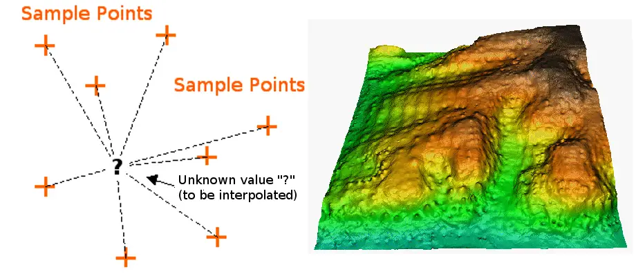
Interpolation is the process of using points with known values or sample points to estimate values at other unknown points. It can be used to predict unknown values for any geographic point data, such as elevation, rainfall, chemical concentrations, noise levels, and so on.

The available interpolation methods are listed below.

Inverse Distance Weighted (IDW)

The Inverse Distance Weighting interpolator assumes that each input point has a local influence that diminishes with distance. It weights the points closer to the processing cell greater than those further away. A specified number of points, or all points within a specified radius can be used to determine the output value of each location. Use of this method assumes the variable being mapped decreases in influence with distance from its sampled location.

The Inverse Distance Weighting (IDW) algorithm effectively is a moving average interpolator that is usually applied to highly variable data. For certain data types it is possible to return to the collection site and record a new value that is statistically different from the original reading but within the general trend for the area.

The interpolated surface, estimated using a moving average technique, is less than the local maximum value and greater than the local minimum value.

IDW interpolation explicitly implements the assumption that things that are close to one another are more alike than those that are farther apart. To predict a value for any unmeasured location, IDW will use the measured values surrounding the prediction location. Those measured values closest to the prediction location will have more influence on the predicted value than those farther away. Thus, IDW assumes that each measured point has a local influence that diminishes with distance. The IDW function should be used when the set of points is dense enough to capture the extent of local surface variation needed for analysis. IDW determines cell values using a linear-weighted combination set of sample points. It weights the points closer to the prediction location greater than those farther away, hence the name inverse distance weighted.

The IDW technique calculates a value for each grid node by examining surrounding data points that lie within a user-defined search radius. Some or all of the data points can be used in the interpolation process. The node value is calculated by averaging the weighted sum of all the points. Data points that lie progressively farther from the node influence the computed value far less than those lying closer to the node.

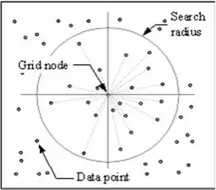
A radius is generated around each grid node from which data points are selected to be used in the calculation. Options to control the use of IDW include power, search radius, fixed search radius, variable search radius and barrier.

Note: The optimal power (p) value is determined by minimizing the root mean square prediction error (RMSPE).

Advantages

• Can estimate extreme changes in terrain such as: Cliffs, Fault Lines.

• Dense evenly space points are well interpolated (flat areas with cliffs).

• Can increase or decrease amount of sample points to influence cell values.

Disadvantages

• Cannot estimate above maximum or below minimum values.

• Not very good for peaks or mountainous areas.

 

 

Natural Neighbour Inverse Distance Weighted (NNIDW)

Natural neighbor interpolation has many positive features, can be used for both interpolation and extrapolation, and generally works well with clustered scatter points. Another weighted-average method, the basic equation used in natural neighbor interpolation is identical to the one used in IDW interpolation. This method can efficiently handle large input point datasets. When using the Natural Neighbor method, local coordinates define the amount of influence any scatter point will have on output cells.

The Natural Neighbour method is a geometric estimation technique that uses natural neighbourhood regions generated around each point in the data set.

Like IDW, this interpolation method is a weighted-average interpolation method. However, instead of finding an interpolated point’s value using all of the input points weighted by their distance, Natural Neighbors interpolation creates a Delauney Triangulation of the input points and selects the closest nodes that form a convex hull around the interpolation point, then weights their values by proportionate area. This method is most appropriate where sample data points are distributed with uneven density. It is a good general-purpose interpolation technique and has the advantage that you do not have to specify parameters such as radius, number of neighbours or weights.

 

 

This technique is designed to honour local minimum and maximum values in the point file and can be set to limit overshoots of local high values and undershoots of local low values. The method thereby allows the creation of accurate surface models from data sets that are very sparsely distributed or very linear in spatial distribution.

Advantages

• Handles large numbers of sample points efficiently.

 

 

Spline

Spline estimates values using a mathematical function that minimizes overall surface curvature, resulting in a smooth surface that passes exactly through the input points.

Conceptually, it is analogous to bending a sheet of rubber to pass through known points while minimizing the total curvature of the surface. It fits a mathematical function to a specified number of nearest input points while passing through the sample points. This method is best for gently varying surfaces, such as elevation, water table heights, or pollution concentrations.

There are two spline methods: regularized and tension.

A Regularized method creates a smooth, gradually changing surface with values that may lie outside the sample data range. It incorporates the first derivative (slope), second derivative (rate of change in slope), and third derivative (rate of change in the second derivative) into its minimization calculations.

Although a Tension spline uses only first and second derivatives, it includes more points in the Spline calculations, which usually creates smoother surfaces but increases computation time.

This method pulls a surface over the acquired points resulting in a stretched effect. Spline uses curved lines (curvilinear Lines method) to calculate cell values.

Choosing a weight for Spline Interpolations

Regularized spline: The higher the weight, the smoother the surface. Weights between 0 and 5 are suitable. Typical values are 0, .001, .01, .1,and .5.

Tension spline: The higher the weight, the coarser the surface and more the values conform to the range of sample data. Weight values must be greater than or equal to zero. Typical values are 0, 1, 5, and 10.

Advantages

• Useful for estimating above maximum and below minimum points.

• Creates a smooth surface effect.

Disadvantages

• Cliffs and fault lines are not well presented because of the smoothing effect.

• When the sample points are close together and have extreme differences in value, Spline interpolation doesn’t work as well. This is because Spline uses slope calculations (change over distance) to figure out the shape of the flexible rubber sheet.

 

 

Kriging

Kriging is a geostatistical interpolation technique that considers both the distance and the degree of variation between known data points when estimating values in unknown areas. A kriged estimate is a weighted linear combination of the known sample values around the point to be estimated.

Kriging procedure that generates an estimated surface from a scattered set of points with z-values. Kriging assumes that the distance or direction between sample points reflects a spatial correlation that can be used to explain variation in the surface. The Kriging tool fits a mathematical function to a specified number of points, or all points within a specified radius, to determine the output value for each location. Kriging is a multistep process; it includes exploratory statistical analysis of the data, variogram modeling, creating the surface, and (optionally) exploring a variance surface. Kriging is most appropriate when you know there is a spatially correlated distance or directional bias in the data. It is often used in soil science and geology.

The predicted values are derived from the measure of relationship in samples using sophisticated weighted average technique. It uses a search radius that can be fixed or variable. The generated cell values can exceed value range of samples, and the surface does not pass through samples.

The Kriging Formula

Kriging is similar to IDW in that it weights the surrounding measured values to derive a prediction for an unmeasured location. The general formula for both interpolators is formed as a weighted sum of the data:

 

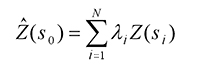
• where:

  Z(s_i) = the measured value at the ith location

  λ_i = an unknown weight for the measured value at the ith location

  s₀ = the prediction location

  N = the number of measured values

In IDW, the weight, λ_i, depends solely on the distance to the prediction location. However, with the kriging method, the weights are based not only on the distance between the measured points and the prediction location but also on the overall spatial arrangement of the measured points. To use the spatial arrangement in the weights, the spatial autocorrelation must be quantified. Thus, in ordinary kriging, the weight, λ_i, depends on a fitted model to the measured points, the distance to the prediction location, and the spatial relationships among the measured values around the prediction location. The following sections discuss how the general kriging formula is used to create a map of the prediction surface and a map of the accuracy of the predictions.

 

 

Types of Kriging

Ordinary Kriging

Ordinary kriging assumes the model

Z(s) = µ + ε(s),

where µ is an unknown constant. One of the main issues concerning ordinary kriging is whether the assumption of a constant mean is reasonable. Sometimes there are good scientific reasons to reject this assumption. However, as a simple prediction method, it has remarkable flexibility.

Ordinary kriging can use either semivariograms or covariances, use transformations and remove trends, and allow for measurement error.

Simple Kriging

Simple kriging assumes the model

Z(s) = µ + ε(s),

where µ is a known constant.

Simple kriging can use either semivariograms or covariances, use transformations, and allow for measurement error.

Universal Kriging

Universal kriging assumes the model

Z(s) = µ(s) + ε(s),

where µ(s) is some deterministic function.

Universal kriging can use either semivariograms or covariances, use transformations, and allow for measurement error.

Indicator Kriging

Indicator kriging assumes the model

I(s) = µ + ε(s),

where µ is an unknown constant and I(s) is a binary variable. The creation of binary data may be through the use of a threshold for continuous data, or it may be that the observed data is 0 or 1. For example, you might have a sample that consists of information on whether or not a point is forest or nonforest habitat, where the binary variable indicates class membership. Using binary variables, indicator kriging proceeds the same as ordinary kriging.

Indicator kriging can use either semivariograms or covariances.

Probability Kriging

Probability kriging assumes the model

I(s) = I(Z(s) > ct) = µ1 + ε1(s)

Z(s) = µ2 + ε2(s),

where µ₁ and µ₂ are unknown constants and I(s) is a binary variable created by using a threshold indicator, I(Z(s) > c_t). Notice that now there are two types of random errors, ε₁(s) and ε₂(s), so there is autocorrelation for each of them and cross-correlation between them. Probability kriging strives to do the same thing as indicator kriging, but it uses cokriging in an attempt to do a better job.

Probability kriging can use either semivariograms or covariances, cross-covariances, and transformations, but it cannot allow for measurement error.

Disjunctive Kriging

Disjunctive kriging assumes the model

f(Z(s)) = µ1 + ε(s),

where µ₁ is an unknown constant and f(Z(s)) is an arbitrary function of Z(s). Notice that you can write f(Z(s)) = I(Z(s) > c_t), so indicator kriging is a special case of disjunctive kriging. In Geostatistical Analyst, you can predict either the value itself or an indicator with disjunctive kriging.

In general, disjunctive kriging tries to do more than ordinary kriging. While the rewards may be greater, so are the costs. Disjunctive kriging requires the bivariate normality assumption and approximations to the functions f_i(Z(s_i)); the assumptions are difficult to verify, and the solutions are mathematically and computationally complicated.

Disjunctive kriging can use either semivariograms or covariances and transformations, but it cannot allow for measurement error.

Advantages

• Directional influences can be accounted for: Soil Erosion, Siltation Flow, Lava Flow and Winds.

• Exceeds the minimum and maximum point values

Disadvantages

• Does not pass through any of the point values and causes interpolated values to be higher or lower then real values.

 

** To have a deep insight on mathematical approach on Kriging please click Kriging a Interpolation Method.

 

 

 

PointInterp

A method that is similar to IDW, the PointInterp function allows more control over the sampling neighborhood. The influence of a particular sample on the interpolated grid cell value depends on whether the sample point is in the cellʼs neighborhood and how far from the cell being interpolated it is located. Points outside the neighborhood have no influence.

The weighted value of points inside the neighborhood is calculated using an inverse distance weighted interpolation or inverse exponential distance interpolation. This method interpolates a raster using point features but allows for different types of neighborhoods. Neighborhoods can have shapes such as circles, rectangles, irregular polygons, annuluses, or wedges.

Trend

Trend is a statistical method that finds the surface that fits the sample points using a least-square regression fit. It fits one polynomial equation to the entire surface. This results in a surface that minimizes surface variance in relation to the input values. The surface is constructed so that for every input point, the total of the differences between the actual values and the estimated values (i.e., the variance) will be as small as possible.

It is an inexact interpolator, and the resulting surface rarely passes through the input points. However, this method detects trends in the sample data and is similar to natural phenomena that typically vary smoothly.

Advantage

• Trend surfaces are good for identifying coarse scale patterns in data; the interpolated surface rarely passes through the sample points.

Topo to Raster

By interpolating elevation values for a raster, the Topo to Raster method imposes constraints that ensure a hydrologically correct digital elevation model that contains a connected drainage structure and correctly represents ridges and streams from input contour data. It uses an iterative finite difference interpolation technique that optimizes the computational efficiency of local interpolation without losing the surface continuity of global interpolation. It was specifically designed to work intelligently with contour inputs.

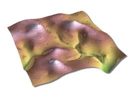
Below is an example of a surface interpolated from elevation points, contour lines, stream lines, and lake polygons using Topo to Raster interpolation.

Topo to Raster is a specialized tool for creating hydrologically correct raster surfaces from vector data of terrain components such as elevation points, contour lines, stream lines, lake polygons, sink points, and study area boundary polygons.

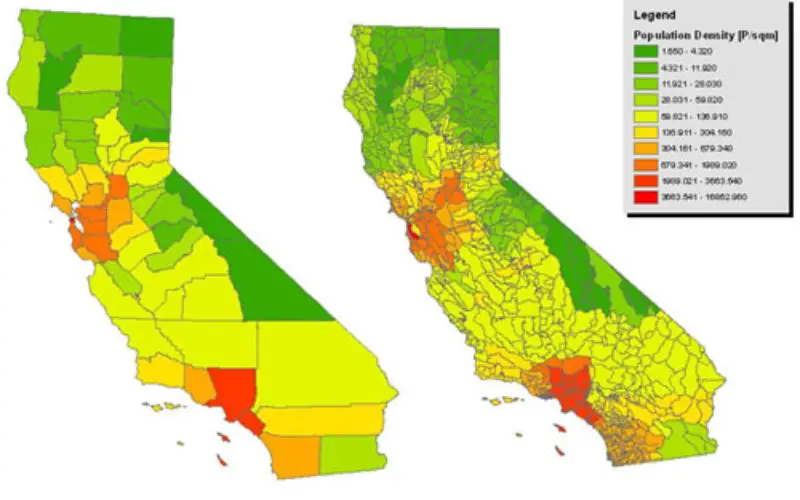
Density

Density tools (available in ArcGIS) produce a surface that represents how much or how many of some thing there are per unit area. Density tool is useful to create density surfaces to represent the distribution of a wildlife population from a set of observations, or the degree of urbanization of an area based on the density of roads.

There are density tools for point and line features in ArcGIS.

 

Related Topics

• What is Interpolation ?

• Classification of Interpolation Techniques.

• Choosing the Right Interpolation Method

 

 

 

References:

University of the Western Cape

ESRI Education Services

IDRRE – Institute for Digital Research and Education

Kriging Interpolation by Chao-yi Lang, Dept. of Computer Science, Cornell University

Pollution models and inverse distance weighting: Some critical remarks by Louis de Mesnard

Overview of IDW – Penn State University